Characterizing the 14-dimensional solutions space of the power market optimization problem

Introduction

Every day in the European power market, electricity prices are set for the next day based on forecasted supply and demand. The intersection of these two curves determines the market-clearing price. Every day, Power Operators have to plan which power plants to turn on the next day to meet the forecasted demand. To decide, they run optimization algorithms to minimize production costs while adhering to both demand requirements and power grid constraints.

In this dynamic market, quantitative traders aim to predict power prices, a task requiring a deep understanding of the parameters influencing the power market optimization problem. That’s where I come into the picture. I’ve helped my team better understand the power grid constraints, building visualization tools and an ML model.

Problem Formulation

Due to physical laws and limited transmission capacities, the power net exportation of each country in Europe is restricted by the grid through this set of constraints:

• \(CB\) represents the set of critical branches (=lines) of the power grid.
• \(Zones\) is the set of zones within the market (France, Belgium..). There are 14 zones, which is why we deal with a 14-dimensional problem.
• \(n_{ex_z}\) stands for the net export of electricity of zone z.
• \(PTDF_{z,cb}\) is the Power Transfer Distribution Factor for zone \(z\) on the critical line \(cb\) (see it as a tool used by system operators to predict how changes in one part of the network will affect the rest of the system).
• \(RAM_{cb}\) represents the Reliability Margin on critical lines (see it as the physical limitation of the line).

The Net Exports satisfying this set of constraints are called the feasible solutions of the constraints set. Noting $N_{ex}$ the 14*1 vectors of possible net exports, the ones that are in the solutions space are defined by:

{ \(N_{ex} \in R^{14} : PTDF.N_{ex} \leq RAM\) }

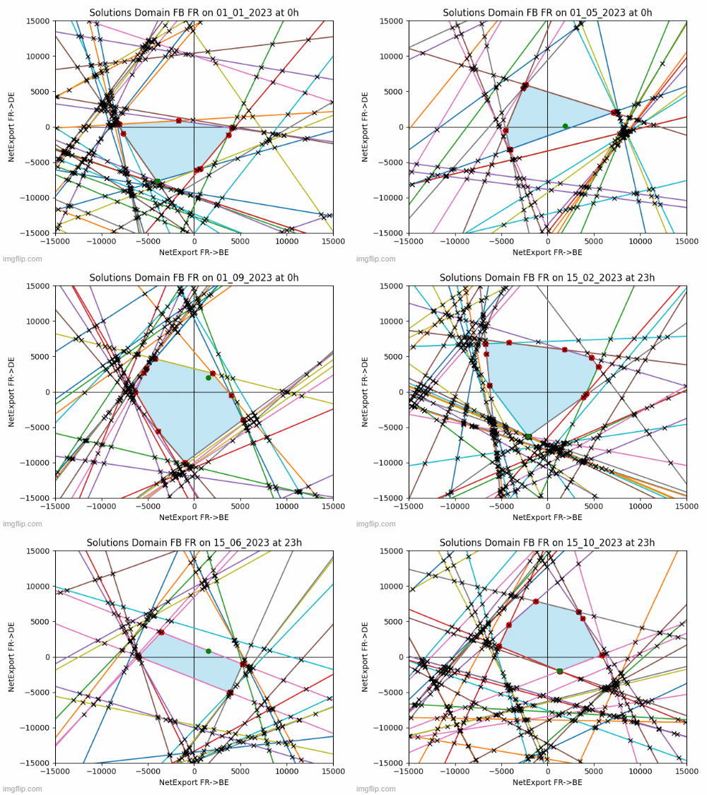
The feasible solutions, or Net Exports, satisfying to these constraints form a convex polyhedron in a 14-dimensional space. Visualizing a 14-dimensional object is not feasible, but we can examine its 2D facets. For example, consider the facet representing net exports between France and Belgium (FR->BE) and France and Germany (FR->DE). I’ve created the animated image below to showcase the evolution of this solution space in 2023. The feasible area is highlighted in blue, with each line representing a constraint. The actual solution is depicted as a green point.

Forecasting the characteristics of the polyhedron over time

The shape of this solution space changes over time, influenced by varying weather conditions which affect both power supply (like wind turbines, dams, solar panels) and demand (such as heating and industrial needs). I developed a Python-based ML pipeline to predict these changes. The project encompassed:

1) Data acquisition from multiple sources via API calls.
2) Data preprocessing and cleaning.
3) Feature engineering and selection.
4) Model selection, training, and evaluation.
5) Deployment in a production environment.

Order of magnitude

There are more than 2000 constraints in the power grid, but Power Operators use a pre-solver to narrow the problem down to about 130 active constraints actually shaping the polyhedron. The size of the matrices “PTDF” is therefore 130*14 i.e each matrix contains 1820 cells to forecast.

Further details

Due to confidentiality, further details on the code and methodology cannot be disclosed at this time. All what is said in this page comes from public data and doesn’t describe the methods used in my company.